Forecasting Gold Prices using ARIMA Model For Time Series

Introduction

Gold is one of the most popular and historical investments. Investors have always been interested in gold prices and have used multiple analysis methods to predict its price over time. In this article, we will discuss the use of the ARIMA model to forecast the price of gold.

What is ARIMA?

ARIMA stands for Auto-Regressive Integrated Moving Average. It is a method for modeling time series data for forecasting. A time series is a sequence of data points indexed in time order. Forecasting refers to predicting future data points in the series.

Loading and Preparing the Data

For this application, we used data from Kaggle. The dataset contains 1,718 rows and 80 columns, spanning from November 18, 2011, to January 1, 2019. The relevant columns for this study are 'Date' and 'Close', representing the date and closing price, respectively.

Splitting data into training and testing sets is standard practice. In this application, we use 80% of the data for training and 20% for testing.

# Split the data into training and testing sets
# Calculate split index
split_index = int(len(data) * 0.8)
                    
# Split the DataFrame
df_train = data.iloc[:split_index]
df_test = data.iloc[split_index:]
                

Stationarity Testing

Stationarity is an important property in time series analysis. A time series is stationary if parameters such as mean and variance do not change over time.

To determine if our time series is stationary, we use the Augmented Dickey-Fuller (ADF) test. This test returns a p-value. If p is less than 0.05, the series is stationary; otherwise, it is not.

from statsmodels.tsa.stattools import adfuller

# Perform Augmented Dickey-Fuller test for stationarity
result = adfuller(df_train['Close'])
print('ADF Statistic:', result[0])
print('p-value:', result[1])
                

In our case, the p-value is 0.489, indicating that our time series is not stationary.

Differencing and Rechecking for Stationarity

Since the time series is not stationary, we cannot directly apply ARIMA. One way to address this is by differencing the time series.

# First differencing
data_diff = df_train['Close'].diff().dropna()
                

After differencing, we recheck if the new time series is stationary using the ADF test. In this case, the series became stationary after the first differencing, meaning the differencing order d = 1.

ACF and PACF Plots to Determine ARIMA Parameters

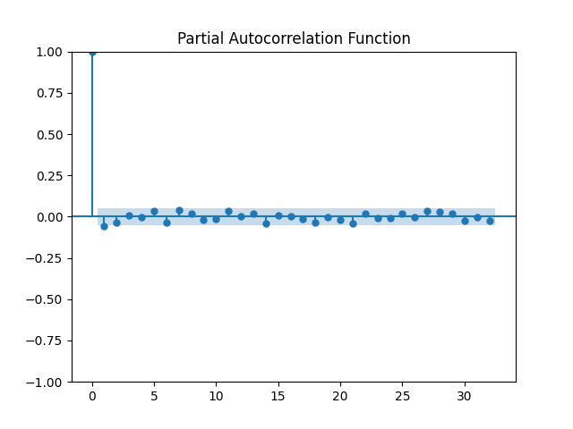
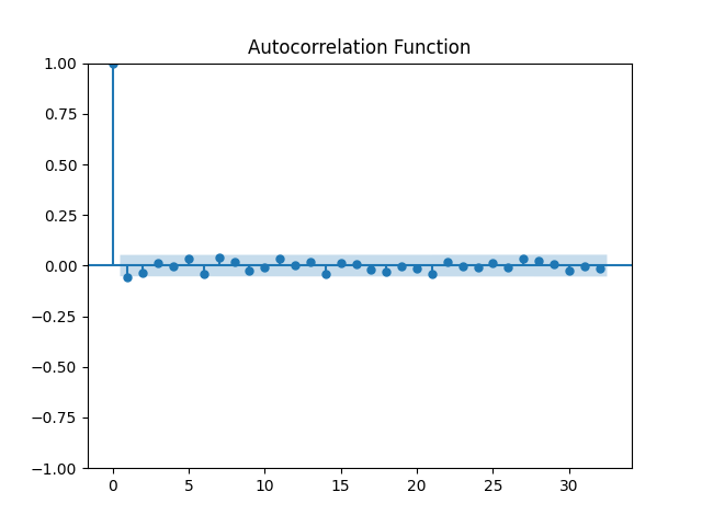
Now, we will plot ACF (Autocorrelation Function) and PACF (Partial Autocorrelation Function) to determine the moving average (q) order and lag order (p), respectively.

From the figures, we conclude that the lag order p = 1 and the moving average order q = 1.

Modeling with ARIMA

After determining the ARIMA parameters (p, d, q), we can proceed to train our model.

# Model parameters determined by inspecting ACF and PACF
p = 1  # lag order
d = 1  # differencing order
q = 1  # moving average order
                    
# Define the ARIMA model
model = ARIMA(data['Close'], order=(p, d, q))
                    
try:
    model_fit = model.fit()
except Exception as e:
    print(f"Model fitting failed: {e}")
    exit()
                

Forecasting and Plotting Results

Now that we have our model trained, we will forecast the testing set using this model.

# Forecast the future values
forecast_steps = len(df_test['Close'])
forecast = model_fit.forecast(steps=forecast_steps)
                

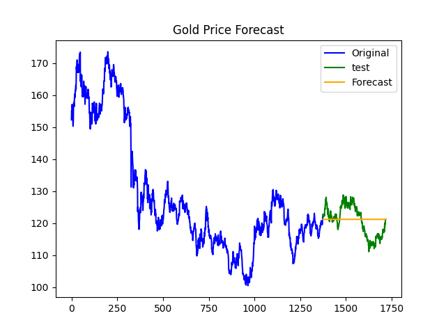
For visual interpretation, we will plot the training set, testing set, and forecasted values.

Evaluating the Model's Performance

By calculating the Mean Absolute Error (MAE), Mean Squared Error (MSE), and Root Mean Squared Error (RMSE), we can evaluate our model. In our case, MAE = 3.9476, MSE = 21.627, and RMSE = 4.650. These errors are relatively low compared to the data values, which range between 100 and 200, suggesting that the model performs well.

In the financial context, making accurate predictions is challenging due to volatility. However, more advanced models, like SARIMA or hybrid models combining ARIMA with machine learning methods, may offer improved performance.